Quick answer
Excel 365 / 2021 / web
Use XLOOKUP
Any direction, exact match by default, built-in not-found.
Excel 2016 / 2019
Use INDEX MATCH
Left-lookup alternative. Works in every version since 2007.
Legacy workbook
Keep VLOOKUP
Hundreds of existing formulas and no appetite to migrate.
VLOOKUP is 39 years old and still works, but if you are writing it today you are choosing the harder, more brittle path for no reason. Here is the upgrade you can make in an afternoon.
The difference between VLOOKUP and XLOOKUP
VLOOKUP searches for a value in the leftmost column of a table and returns a value from a column to the right - always to the right, never the left. XLOOKUP searches any column or row and returns a result from any other column or row, in any direction. The lookup range and the return range are independent. That one architectural difference cascades into everything: no more counting columns, no more #N/A propagation, no more broken formulas when someone inserts a column.
The same job, side by side
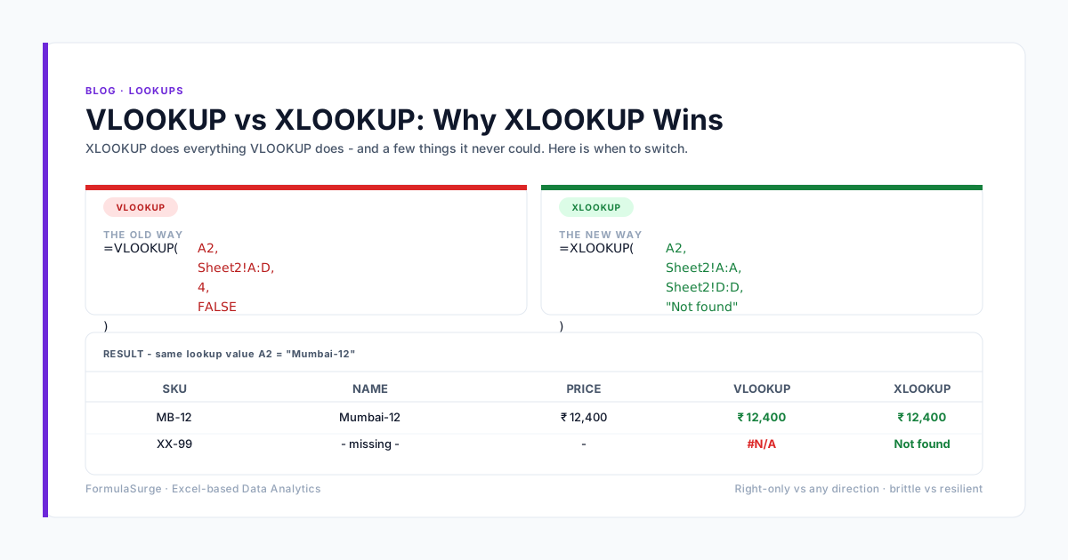
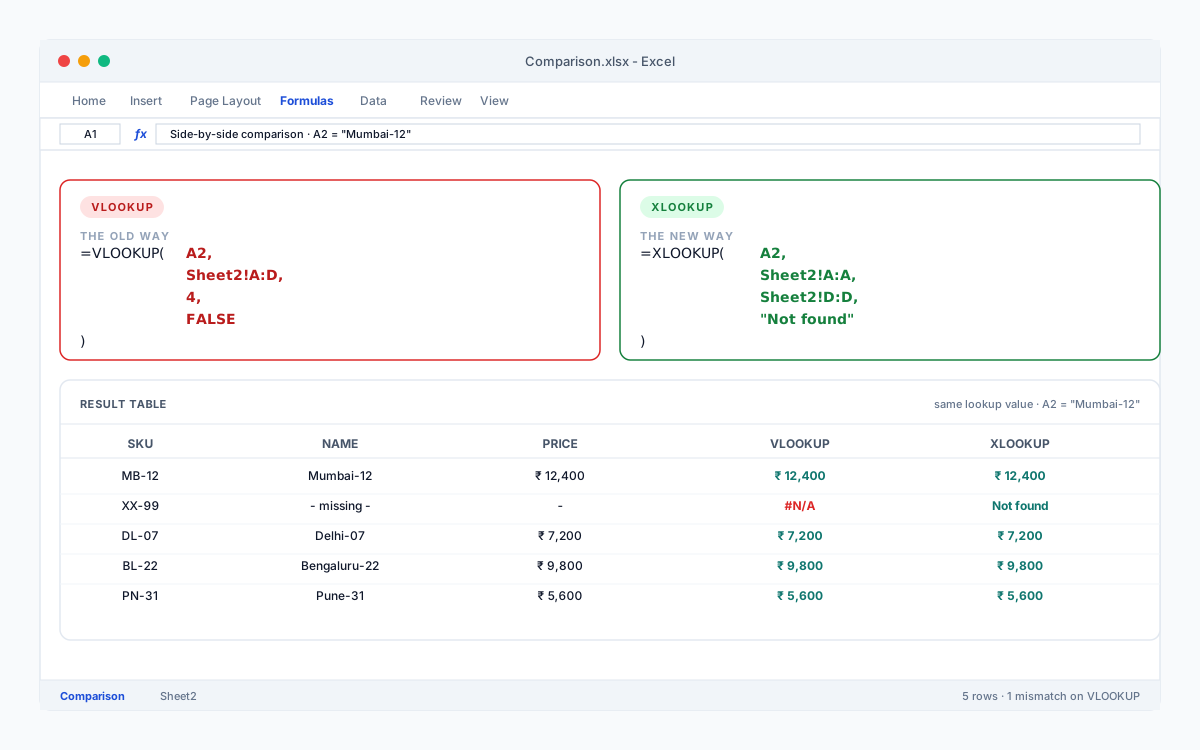
To pull a customer's region from a customer table given their ID, the two formulas are:
VLOOKUP(A2, Customers!A:D, 4, FALSE)- column 4 must always be region.XLOOKUP(A2, Customers!A:A, Customers!D:D, "Unknown")- readable, robust, and returns "Unknown" instead of#N/A.
Where XLOOKUP clearly wins
| Feature | VLOOKUP | XLOOKUP |
|---|---|---|
| Direction of lookup | Always looks right. Need the column left of the key? Use INDEX/MATCH instead. | Looks in any direction. The lookup range and the return range are independent. |
| Default match mode | Approximate by default. A sorted table out of order silently returns the wrong row. | Exact match by default. You have to ask for approximate, and you say it explicitly. |
| Missing values | Returns #N/A on a miss - which then propagates through every formula that uses it. | Has a built-in fourth argument for the not-found value: =XLOOKUP(key, range, result, "Not found"). |
| Column index fragility | Hard-codes a column number (3, 4, 7). Insert a column in the source and every formula breaks. | Takes a return range, not a number. Insert a column and nothing breaks. |
| Multi-cell return | Returns one cell. Spilling several columns needs a wrapper. | Returns an array - pass a multi-column range and it spills them all. |
The migration is mechanical
For every VLOOKUP in your workbook, replace the column number with the actual range of the return column, and add a not-found message as the fourth argument. That is it. You can do it with Find & Replace on a whole sheet if you keep your ranges named.
When VLOOKUP is still fine
Honestly: almost never. The only argument for keeping VLOOKUP is "I am sending this file to someone on Excel 2016 or older". If you control the audience, switch. If you do not, wrap the XLOOKUP in IFERROR for safety, but the modern function is still the better default.
XLOOKUP syntax and arguments - what matters for production workbooks
XLOOKUP takes three required arguments and three optional ones. The signature is:=XLOOKUP(lookup_value, lookup_array, return_array, [if_not_found], [match_mode], [search_mode]). The first three are the same as VLOOKUP - what to look up, where to look, what to return. The optional three are where XLOOKUP earns its keep.
if_not_foundis the most-used optional argument. It kills the #N/A propagation problem - pass "Not found", 0, or any fallback value. Omit it and XLOOKUP behaves like VLOOKUP on a miss.
match_mode defaults to exact match (0). The other options - next-smaller (-1), next-larger (1), and wildcard (2) - are useful but rarely needed in finance workbooks. Most production XLOOKUPs use the default.
search_mode defaults to first-to-last linear (1). Set it to 2 (binary search ascending) or -2 (binary search descending) on 100K+ row ranges for 2–5x speedup - but the data must be sorted or XLOOKUP returns the wrong row silently. Most teams never use this; on the workbook sizes that show up in our audits, the default is fast enough.
Most XLOOKUP formulas in production are short - three arguments, a not-found value, done. The optional arguments exist for the edge cases. If a model has many XLOOKUPs with custom match_mode or search_mode, that is usually a sign the data shape is wrong and needs cleanup before the lookup layer is reliable.
Why migrating VLOOKUP to XLOOKUP is harder than it looks
On paper the migration is mechanical: replace the column number with a range, add a not-found argument, split the table_array in two. On a real-world workbook with 200+ formulas, three quarters of the job is the work around the migration, not the migration itself.
The first problem is naming. VLOOKUP references columns by number (3, 4, 7). XLOOKUP references them by range. If the source table is a flat range, finding the right column range is manual - and a column inserted between B and D silently breaks every formula. The fix is to convert the source to a Table first, then point every formula at structured references.
The second problem is the not-found behaviour. VLOOKUP returns #N/A on a miss. XLOOKUP returns whatever you pass in the fourth argument - or #N/A if you omit it. Most legacy workbooks have IFERROR wrappers around every VLOOKUP. The migration is the moment to delete those wrappers and use the built-in argument, but every team we work with forgets and ends up with double-wrapped formulas that swallow the not-found message.
The third problem is audit. A 200-formula workbook that gets a Find & Replace on the function name has to be verified cell by cell. The argument shapes are different (one combined range vs two ranges, optional fourth argument), so the regex catches the name but the formulas still need a hand review. We typically spend 1–2 working days on a 200-formula workbook: half on the migration, half on verifying the result.
XLOOKUP vs INDEX MATCH - which should you actually use?
INDEX MATCH is the older left-lookup alternative to VLOOKUP. It works in every version of Excel since 2007. The question of XLOOKUP vs INDEX MATCH comes up most often when the audience uses older Excel or a system that exports to CSV.
The formulas do the same job - look up a value in one column and return from another:
=XLOOKUP(A2, Customers!A:A, Customers!D:D, "Unknown")=INDEX(Customers!D:D, MATCH(A2, Customers!A:A, 0))
The XLOOKUP version is shorter, has the built-in not-found argument, and reads cleanly. The INDEX MATCH version works in Excel 2016 and older.
When to pick each:
- Pick XLOOKUP when your audience is on Excel 2021 / Microsoft 365 / Excel for the web. Most enterprise users today. Shorter formula, clearer intent, built-in not-found.
- Pick INDEX MATCH when you are sending the file to Excel 2016 / 2019 users or to a system that exports to CSV and runs the formula in a legacy Excel runtime. INDEX MATCH also wins on the most obscure left-lookups where XLOOKUP is not available.
- Pick VLOOKUP almost never. The only case is a legacy workbook with hundreds of existing formulas and no appetite to migrate.
On speed, INDEX MATCH and XLOOKUP are similar on normal-sized ranges. On 100K+ row ranges, XLOOKUP with binary search is faster - useful for the few workbooks that need it. For most finance workbooks, the choice between XLOOKUP and INDEX MATCH is about the audience, not the speed.
Related reading
- SUMPRODUCT - the function that replaces five for the next lookup-style problem you will hit.
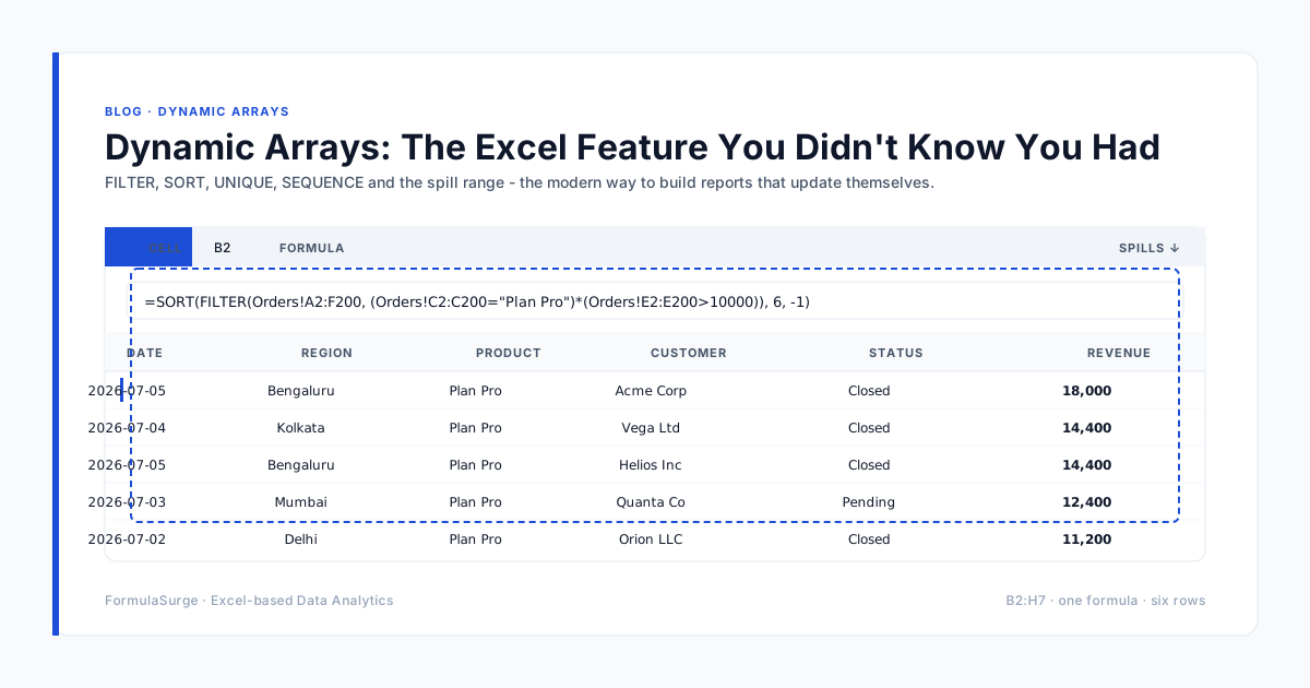
- Dynamic Arrays - the Excel feature you didn't know you had because XLOOKUP spills - and you will want to know how.
- 10 Excel functions every analyst should know for the rest of the formula toolkit behind every dashboard.