ABC analysis is the operational application of Pareto to inventory. The pattern is: classify SKUs by contribution, drive different policies for each class, and watch the working capital drop. The seven steps below are the standard pattern we ship on every inventory engagement. The pattern is also the foundation of the reorder point calculator on the Tools page.
The seven steps
01
Pull 12 months of sales by SKU
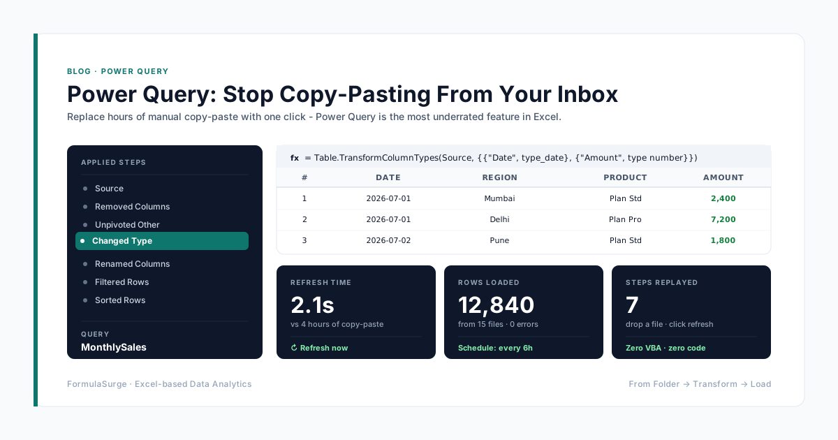
Export the sales register for the last 12 months. Each row is an invoice line with SKU, quantity, revenue, and ideally margin. The data lands in a Table (Ctrl+T). The senior uses Power Query to ingest the export and merge with the SKU master to get the cost and margin.
02
Sum revenue and margin by SKU
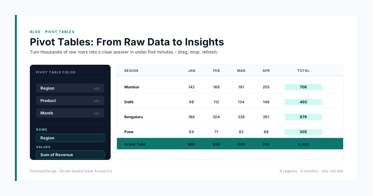
Pivot Table or SUMIFS by SKU. The output is one row per SKU with annual revenue, annual margin, and annual quantity. The senior uses a Pivot Table for speed and a SUMIFS pattern for the formula-driven version. The Pivot Table is auditable; the SUMIFS is reproducible.
03
Sort descending by contribution
Sort the table by revenue or margin descending. The top row is the highest-contribution SKU; the bottom row is the lowest. The senior uses margin by default. The sort sets up the cumulative calculation that follows.
04
Calculate cumulative % of total
Running total of contribution divided by the grand total. The senior uses =SUM($B$2:B2)/SUM($B$2:$B$N) as the running percentage. The formula fills down and the running total reaches 100% on the last row.
05
Assign A/B/C by threshold
IFS or nested IF on the cumulative %. A = cumulative <= 80%, B = cumulative <= 95%, C = everything else. The senior uses an IFS for readability. The classification becomes a column on the table.
06
Pivot to summarise by class
Pivot Table with A/B/C as rows and SKU count, revenue, margin, and quantity as values. The summary table is the input to the operational policy. The senior adds a chart - a column chart with the class on the x-axis and the count on the y-axis.
07
Plot the cumulative curve
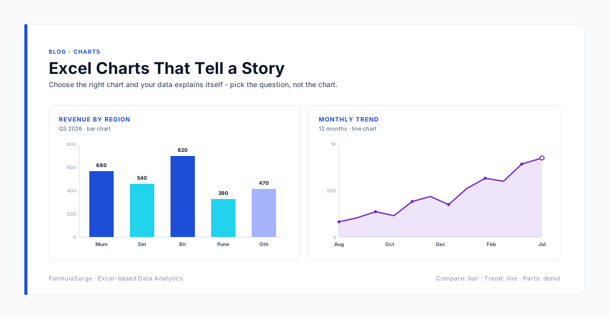
Line chart with the SKU rank on the x-axis and the cumulative % on the y-axis. The classic ABC curve. The knee of the curve is the boundary between A and B; the second knee is the boundary between B and C. The senior uses this chart to communicate the classification to the operations team.
The A/B/C policy
The classification is useless without the policy. The standard policy below is the one we ship on most engagements. Tune the thresholds and the review cadence to match the business.
A items
~20% of SKU countContribution: Top 80% of contribution
Policy: Weekly reorder review, tight safety stock, monthly physical count
B items
~30% of SKU countContribution: Next 15% of contribution
Policy: Bi-weekly reorder review, moderate safety stock, quarterly physical count
C items
~50% of SKU countContribution: Bottom 5% of contribution
Policy: Monthly reorder review, generous safety stock (or none), annual physical count
From ABC to reorder policy
The ABC classification is the input to the reorder policy. For A items, the reorder point is the lead-time demand plus a small safety stock (calculated from the standard deviation of lead-time demand). For B items, the safety stock is larger. For C items, the safety stock is often zero and the reorder is a fixed order quantity on a fixed cadence. The reorder point calculator on the Tools page implements the A-item formula. The senior builds the B and C item policies on the same workbook, with the classification driving the formula choice.
What the operational impact looks like
The typical ABC engagement cuts working capital by 15-25% in the first six months. The mechanism is: the A items get reviewed weekly (was monthly), the B items get reviewed bi-weekly (was quarterly), the C items get a generous safety stock and a quarterly review (was monthly). The reorder quantity drops on the A items, the safety stock drops on the B items, and the obsolescence drops on the C items. The senior ships the classification in two weeks, the policy in the following two weeks, and the working capital impact shows up in the next quarter.