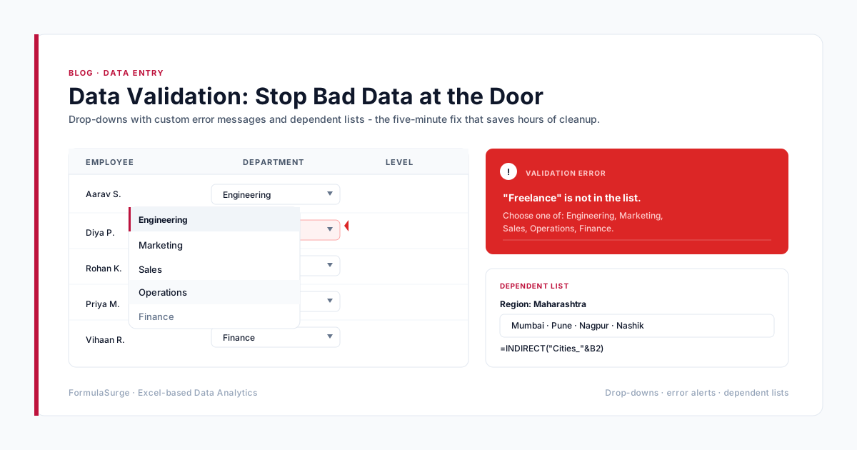
Most data-cleaning work in Excel is fixing typos that should never have been typed. A five-minute Data Validation setup on the input sheet can save five hours of cleanup per quarter. Here is the version we put in front of every client team.
What Data Validation actually does
Data Validation lives on the Data tab and controls what a cell will accept. When a user types something the rule rejects, Excel blocks it (or warns, depending on the style you choose). It does not format or color - it gates the input itself. The cell will never hold an invalid value, which means everything downstream - pivots, SUMIFS, charts - is built on clean data by construction.
Four setups we use on every intake sheet
- 1
Drop-downs for any finite list
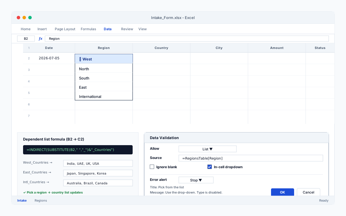
Region, product, status, payment method - anything drawn from a known set. Data > Validation > List, point at the range. Typing is now impossible; the wrong value is now impossible.
- 2
Numeric bounds on quantities and amounts
Whole number between 1 and 1,000,000. Decimal greater than 0. Date after 2024-01-01. The five-minute setup catches typos that would otherwise survive until month-end.
- 3
Dependent lists that change with the parent
Pick a region from one drop-down, the country list updates. Pick a country, the city list updates. One small INDIRECT formula in the source range and your entry form becomes self-correcting.
- 4
Error messages that teach
The default Excel error ("The value you entered is not valid") teaches nothing. Use the Input Message tab to show instructions and the Error Alert tab to write a specific correction: "Enter a date in 2026 in the format dd-mmm-yyyy".
How to save data validation rules and copy them across sheets
Data Validation rules live on cells, not in a central library. Copying a cell copies the rule along with the formatting - Ctrl+C, Ctrl+V. But if you need to copy only the validation rule without overwriting existing values or formatting, use Paste Special: right-click, Paste Special, choose Validation. Excel applies the rule and leaves everything else alone.
To find every cell that has data validation on a sheet: Home > Find & Select > Go To Special > Data Validation > All. Excel highlights every validated cell on the active sheet. To select only the cells that share the same rule, choose Same instead of All. From there, you can copy the rule set in one paste operation.
The most reliable way to save a data validation rule for reuse is to define it on a Table column, not on a range. When new rows are added to a Table, Excel extends the validation to the new rows automatically - no copy-paste step, no forgotten cells, no gap in the gate. Combined with a named range for the drop-down source, the rule becomes self-maintaining.
Use Tables, not ranges, for the source lists
When the drop-down source is a range, the list is frozen the day you set it up. When the source is a Table, adding a new region or product updates the drop-down automatically. Same idea for the INDIRECT-based dependent lists - point them at named ranges on a hidden sheet, and the lists scale without anyone touching the validation.
The test that proves it is working
Try to enter an invalid value. If Excel lets it through, the rule is not strict enough - change Style from "Warning" or "Information" to "Stop". Stop is the only style that actually protects the data; the others just nag.
Why data validation on real workbooks is harder than the documentation suggests
Data Validation looks simple - pick Allow from a drop-down, fill in the Source, click OK. On a typical real-world workbook, three problems show up within an hour.
The source list is in the wrong place. Most workbooks keep the drop-down source as a flat range on the same sheet as the data entry. Two months later, the source has 200 rows, the entry sheet has 5,000 rows, and someone has inserted a row in the source and broken every drop-down. The fix is to move the source to a hidden Lists sheet and reference it as a named range or a Table column - then it never breaks.
The validation does not survive copy-paste. A team member copies a column with the validation and pastes it into a new sheet. The validation comes along, but the named-range reference points at the old sheet, which the new sheet cannot see. Drop-downs go blank. The fix is structured references (Table columns), which move with the data.
The default error message teaches nothing.Every workbook we audit has dozens of validation rules with the default "The value you entered is not valid" error. Users click OK, type the wrong value again, and the rule eventually gets deleted because "nobody uses it anyway". The fix is a custom Error Alert on every hard rule, written for the actual user, in the actual words that explain what to type.
These three fixes - source-on-Lists, structured references, custom error messages - are the difference between a workbook with validation that protects data and a workbook with validation that everyone ignores. Most teams that try to DIY this stop after one rule and never come back.
What a senior Excel consultant actually delivers for an intake sheet
A production-grade intake sheet has four layers:
- A hidden Lists sheet with one column per category (Region, Country, Product, Status, Payment Method). Each column is a Table, so adding a row updates every drop-down automatically.
- Named ranges or structured references pointing at each Table column. Drop-downs reference the name, not the cell, so the source can move without breaking anything.
- Dependent drop-downs via INDIRECT for Region → Country → City. One source of truth, three cascading lists. The pattern scales to N levels.
- Custom Input Message and Error Alert on every hard rule (Stop style). The user sees a specific instruction when they click the cell and a specific correction when they type the wrong value.
Most intake sheets have none of these layers. The validation that exists is broken, the error messages are the default ones, and the sources are flat ranges that break on first edit. We deliver all four layers in a single engagement - typically 1–2 working days for a sheet with 10–15 drop-downs. The team that owns the sheet afterwards can add a new category by typing one row into the Lists sheet; the drop-down updates itself.
Data validation with custom formulas (the advanced gate)
When the built-in validations (Whole Number, Decimal, List, Date, Text Length) are not enough, the Custom validation type lets you write a formula that returns TRUE (valid) or FALSE (invalid). Three useful patterns:
- Prevent duplicates in a column. Custom formula:
=COUNTIF($A$2:$A$1000, A2) = 1. The first occurrence is allowed; the second is blocked. - Require a value when another cell is filled. Custom formula:
=OR(A2="", B2<>""). If A2 has a value, B2 must also have one. - Limit input to business hours or weekdays. Custom formula:
=AND(WEEKDAY(A2, 2) <= 5, HOUR(A2) >= 9, HOUR(A2) < 17). Only weekdays between 9am and 5pm.
Custom formulas run on every entry, so keep them cheap. Avoid array operations, VLOOKUP into large ranges, and volatile functions like INDIRECT unless necessary. On ranges above a few thousand cells, the validation rule itself can slow data entry. The right answer on a real workbook is usually fewer hard rules and more downstream validation in Power Query or a checks tab - the gate at the cell is one of several layers, not the only one.