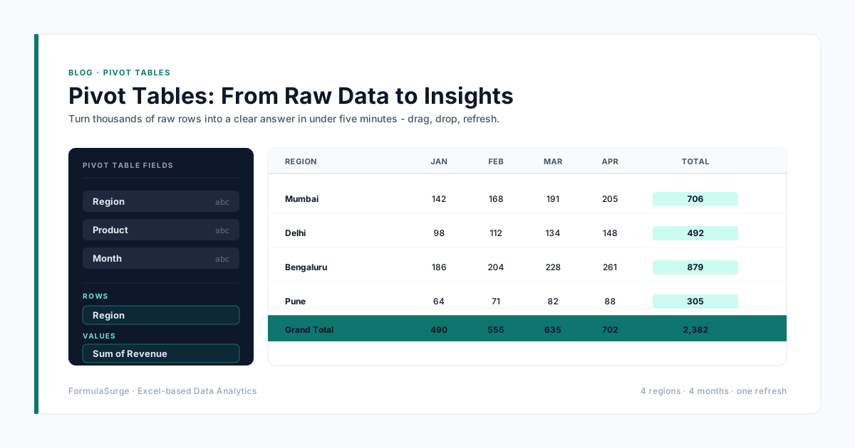
SUMIFS is the single most useful formula in any finance analyst's toolkit. The function sums a range by one or more criteria and handles dates, numbers, text, and wildcards cleanly. Master the four patterns below and you can build 80% of the totals in any finance dashboard without helper columns, without SUMPRODUCT, and without a Pivot Table.
The four patterns
Monthly totals
SUMIFS(amounts, dates, ">="&A1, dates, "<"&EOMONTH(A1,0)+1) sums everything in the current month. A1 is the first of the month. EOMONTH(A1,0)+1 is the first of next month - the < comparison is exclusive, so the formula excludes next month automatically.
=SUMIFS(amounts, dates, ">="&A1, dates, "<"&EOMONTH(A1,0)+1)
YTD totals
SUMIFS(amounts, dates, ">="&DATE(YEAR(TODAY()),1,1)) sums everything from 1 January of the current year. The DATE function is the cleanest way to construct the year start - no manual string concatenation, no leap-year edge cases.
=SUMIFS(amounts, dates, ">="&DATE(YEAR(TODAY()),1,1))
By region and category
SUMIFS(amounts, region, A1, category, B1) sums by two criteria. The function supports up to 127 criteria pairs; in practice, two to four is the maximum that still reads cleanly. Beyond four, the formula is unreadable and the senior should switch to a Pivot Table or a Power Pivot DAX measure.
=SUMIFS(amounts, region, A1, category, B1)
Wildcard match
SUMIFS supports * and ? wildcards in text criteria: SUMIFS(amounts, product, "*Excel*") sums anything with Excel in the product name. The wildcard is case-insensitive. Use ? for single-character wildcards ("A?C" matches ABC, AXC, etc.).
=SUMIFS(amounts, product, "*Excel*")
OR logic with SUMIFS
SUMIFS is AND-only. For OR, two patterns. The first is to add two SUMIFS together - the cleanest for two or three conditions on the same column. The second is SUMPRODUCT with an array - for OR across multiple columns, weighted averages, or counts that SUMIFS cannot do.
=SUMIFS(amounts, region, "North") + SUMIFS(amounts, region, "South")
=SUMPRODUCT((region="North")+(region="South"))*amounts)
The four mistakes to avoid
Sum range and criteria range sizes differ
If sum_range is C2:C1000 and criteria_range is B2:B500, SUMIFS silently truncates. The fix: every range is the same size and starts on the same row. The safest pattern is to convert all data to a Table (Ctrl+T) and use structured references.
Mixing absolute and relative references
If the criteria cell is a relative reference and you copy the formula down, the criteria moves with the formula. The fix: lock the criteria with $ signs (=SUMIFS(amounts, dates, ">="&$A$1, dates, "<"&EOMONTH($A$1,0)+1)).
Date as text in the criteria
If the date in the criteria cell is stored as text, SUMIFS treats it as a string and returns 0. The fix: format the criteria cell as Date and use =DATE(2026,1,1) or a cell reference. Never type a date as "1/1/2026" - Excel interprets the locale inconsistently.
Using SUMIFS where the data is filtered
SUMIFS does not respect the SUBTOTAL/AutoFilter logic. If you filter the data and then SUMIFS, the formula still sums the entire range. The fix: use AGGREGATE or a Pivot Table for filtered totals. SUMIFS is for the whole range, not the visible cells.
SUMIFS vs SUMPRODUCT vs Pivot Table
The three tools overlap. SUMIFS is the right tool for one or two totals on a small range (under 100K rows). SUMPRODUCT is the right tool for OR logic, weighted averages, and multi-column conditional counts. Pivot Table is the right tool when the reader needs to slice the data dynamically with Slicers. The senior uses all three. The junior uses SUMIFS for everything and ends up with a 30-tab workbook full of formulas that all return the same number.