There is a function in Excel that is older than pivot tables, faster than five helper columns, and almost no analyst uses on purpose. SUMPRODUCT has been in Excel since 1985, and it is the one function that quietly does the work of five. The reason it stays under the radar is that the name sounds like a single job - sum the products of two ranges. In practice, it is a small engine for array math, and that is the entire trick.
The mental model, in one sentence
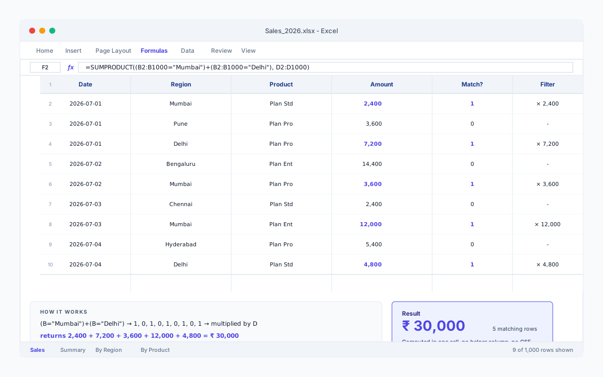
SUMPRODUCT takes one or more arrays of the same shape, multiplies the matching elements, and returns the sum. That is it. Every clever use of SUMPRODUCT is a rearrangement of that one sentence - usually by feeding it arrays of TRUE/FALSE values, which become 1/0 when multiplied. A row that fails the condition becomes 0; a row that passes becomes 1; the amount column multiplied by 1 stays, multiplied by 0 disappears.
Once that lands, the function stops looking like a trick and starts looking like the cleanest way to express a conditional sum. The formula on the screen looks like English, runs in one cell, and survives almost any change to the source data.
The five jobs it replaces
SUMIFS with OR
SUMIFS is AND-only - it cannot say "Mumbai or Delhi" without an array constant. SUMPRODUCT adds the two conditions, then multiplies by the amount column. One cell, no helper column, no spilling.
=SUMPRODUCT((Region="Mumbai") + (Region="Delhi"), Amount)
COUNTIFS with multiple ranges
Count rows that match every condition across four columns. Each condition becomes a 1/0 array; the product is the count of rows that match all four. Try building this with COUNTIFS - you will end up with a nested mess.
=SUMPRODUCT((Region="Mumbai") * (Product="Plan Pro") * (Channel<>"Partner") * (Amount>0))
Weighted average
AVERAGEIF does not take a weight. There is no other built-in way to compute a weighted average of price across line items. SUMPRODUCT multiplies the two arrays, then divides by the sum of weights. Two arguments, one cell, done.
=SUMPRODUCT(Qty, Price) / SUM(Qty)
Conditional max or min
MAXIFS exists in newer Excel, but the SUMPRODUCT version works in every version since 2007. The trick: multiply the values by 1/0, and the unmatched rows become 0 - MAX picks the largest of the kept rows. Wrap in array entry for older Excel.
=MAX((Region="Mumbai") * Amount)
Conditional sum with a divisor
Average revenue per deal in a region, ignoring the zero-qty header rows. SUMIFS would let you sum and count separately, but dividing them as one expression means the formula is harder to break when the source changes.
=SUMPRODUCT((Region="Mumbai") * Amount) / SUMPRODUCT((Region="Mumbai") * (Qty>0))
The two gotchas that bite everyone
Most SUMPRODUCT failures come from one of two places. Both have a one-line fix; the trick is knowing to look for them.
- 1
Booleans need to become numbers
When two booleans are added (with +), Excel coerces them to 1/0 automatically. When they are multiplied (with *), the same coercion happens. The problem is when you compare the result to a number - wrap the condition in double-negation (=-- (condition)) if you want a guaranteed number.
- 2
Dates need to be wrapped
=SUMPRODUCT((Date>=DATE(2026,7,1)) * Amount) works; =SUMPRODUCT((Date>="2026-07-01") * Amount) is fragile because Excel sometimes treats the string as a date, sometimes as text. Always use DATE() inside SUMPRODUCT - it is the only safe pattern.
Delete the helper column
Next time you are about to add a helper column - a 1/0 flag, a weighted value, a transformed amount - stop and write the SUMPRODUCT instead. Five minutes later, the helper column is gone, the formula is shorter, the workbook is harder to break, and you have one less thing to explain to the next person who opens the file. SUMPRODUCT rewards the people who learn it well with reports that are auditable in a single glance.